Prune manual

1. Introduction
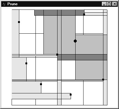
2. The Control Window
3. Mouse Commands
4. Examples

Introduction

This program is used for investigating pruning fronts in Smale's horseshoe. The paper "How to prune a horseshoe" by A. de Carvalho and T. Hall gives a survey of the mathematical background. The program has facilities for plotting periodic, homoclinic, and heteroclinic orbits in the horseshoe, and for calculating maximal symmetric pruning disks with respect to such orbits. The figures created using the program can be saved in internal format, printed, or exported as eps files.

The facilities provided by the program are accessible either via the buttons in the control window, or through pop-up menus activated by right-clicking at strategic points. Note that it is also possible to resize the main display window - this can be useful when running multiple instances of the program simultaneously. A good way to start learning how to use the program would be to work through the simple examples presented at the end of this manual.

The program was written during the course of a research project, with new features added as they became necessary. As such, we weren't always worried about fixing problems which no longer affected us, or with making the user interface as straightforward or as general as possible. Please bear this in mind if you use the program. Please send bug reports to Toby Hall.

Control Window

The following buttons are available in the control window:

Grid
Grid To Front / Back
New Orbit
New Periodic Orbit
New Periodic Point
Open out Disk
Clear All
Zoom Out
Set Title
Print
Save
Load
Export EPS
< and >

Grid

Grid lines (which are segments of the unstable and stable manifolds of the fixed point of code 0) can be displayed to divide the sphere on which the horseshoe acts into equally sized regions. When a number n is selected in the Grid edit box, the sphere is divided into 2^n regions of equal size in both horizontal and vertical directions. n is constrained to lie between 0 and 8.

Right-clicking on a grid intersection brings up a pop-up menu .

Grid To Front / Back

By default, the grid lines are drawn beneath any pruning disks, and hence are obscured by them if the disk is shaded. Clicking this button brings the grid lines to the front. Clicking it again sends them to the back.

New Orbit

Clicking this button brings up a dialog box for entry of a new heteroclinic orbit.A single point of the orbit with code s^\infty q . p r^\infty should be specified, together with the number of points in its forward and backward orbit to be plotted. The words p, r, q, and s should be entered in the Forward Orbit Prefix, Forward Orbit Repeat, Backward Orbit Prefix, and Backward Orbit Repeat edit boxes respectively. The points on the orbit to be plotted are specified in the From and To edit boxes (note that the range specified need not include 0, so the heteroclinic point specified need not itself be plotted). The size, style (solid square, empty square, solid circle, or empty circle), and colour of the plotted points can also be specified.

New Periodic Orbit

Clicking this button brings up a dialog box for entry of a new periodic orbit. The code c_P of the orbit should be entered in the Code edit box. The size, style (solid square, empty square, solid circle, or empty circle), and colour of the orbit points can also be specified.

New Periodic Point

Clicking this button brings up a dialog box for entry of a single periodic point to be plotted. In order to plot the point c^\infty . c^\infty, enter the word c in the Code edit box. The size, style (solid square, empty square, solid circle, or empty circle), and colour of the plotted point can also be specified. Note that this facility is intended solely for producing diagrams: single periodic points do not interact properly with opening out pruning disks, or with other features in the program.

Open out Disk

Clicking this button brings up a dialog box for "opening out" a maximal symmetric pruning disk of specified depth, relative to any orbits and other pruning disks which have been plotted. A word w should be entered in the Word edit box. The program then displays a pruning disk which is symmetric about the vertical centre line of the horseshoe, extends from the top of the horseshoe down to the vertical coordinate w0^\infty, and which is as wide as possible subject to the constraints: i) its interior contains no plotted orbit points; and ii), it doesn't violate the pruning conditions, either with respect to itself or with respect to any other plotted pruning disks.

Note that since the image of the vertical centre line is the right edge of the horseshoe, this is equivalent to opening out a maximal pruning disk of specified height which extends from the right edge of the horseshoe and is symmetric about the horizontal centre line.

The number of forward and backward iterates of the pruning disk to be displayed can be selected in the From and To edit boxes. Note that the range does not need to include 0, so the original disk itself need not be plotted. By default, only an initial segment of each pruning disk image is plotted, extending from its vertices to the first time it crosses the edge of the horseshoe (this is because it is the position of vertices which is most important). Checking the Show Strips check box causes each disk image to be plotted in its entirety. Note that F^n(pruning disk) has a very long boundary if n is far from zero, so choosing this option is a mistake if the values in the From and To edit boxes are large (e.g. their default values of -20 and 20): the program will appear to hang - when it does recover, the whole plotting region will be very black. Moreover, these extended pruning disk images are not filled and/or shaded properly.

The boundary colour, boundary width, fill colour, and fill style (clear, solid, or hatched in various ways) can also be specified.

Clear All

Clicking this button deletes all plotted orbits and pruning disks.

Zoom Out

Clicking this button returns the display region to an unzoomed state. See Zooming in .

Set Title

Clicking this button makes it possible to select a title for the display window. This can be helpful if several instances of the program are running simultaneously. The title is not saved when the Save button is used.

Print

Clicking this button causes the display region to be printed. This may not work properly with all printers.

Save

Clicking this button brings up a Save dialog box for saving the state of the program. The default extension is .pru

Load

Clicking this button brings up a Load dialog box for loading a previously saved .pru file.

Export EPS

Clicking this button brings up a Save dialog box for exporting the contents of the display window in eps format. Note that the exported eps file is not in colour: coloured pruning disks and orbit points are converted to an "appropriate" grayscale, which is probably quite inappropriate. Hatching of pruning disks is also not exported. When creating a figure destined for export, it is therefore advisable to stick to grayscale, and to choose the fill style of pruning disks to be either solid or clear.

< and >

These buttons become available when an orbit or pruning disk is highlighted. They cause the highlighted point of the orbit, or disk in the orbit of pruning disks, to be advanced or withdrawn one step along the orbit. This is a useful feature for understanding the action of F on the orbit or disk.

Mouse Commands

Pop-up menus appear when the right mouse button is clicked on grid intersections, orbit points, or vertices of pruning disks. The menu items depend on which of these has been clicked, and also on whether or not the point clicked is on the unstable manifold of the fixed point of code 0. Dragging with the left mouse button also causes the window to zoom in to the region selected.

Zooming in
Grid point menu (these commands are also available in the Pruning disk menu, and in the orbit menu if the orbit is on the unstable manifold of 0).
Orbit menu
Pruning disk menu

Zooming in

Left-click and drag to select a rectangular region to zoom in on: a pop-up menu appears asking you to confirm the zoom. The rectangular region selected is reshaped to a square, which is outlined with a dashed red line. Zooms can be carried out successively. Use the Zoom Out button to return to an unzoomed state.

Grid point menu

Open Out Disk
Place Orbit

Open Out Disk

Selecting this item causes the Disk Entry dialog box to be displayed, with the vertical coordinate of the clicked point in the Word edit box.

Place Orbit

Selecting this item causes the Orbit Entry dialog box to be displayed, with the coordinates of the clicked point preselected. It therefore makes it possible to plot the orbit containing the clicked point.

Orbit menu

Edit Orbit
Delete Orbit
Highlight Orbit

If the orbit lies on the unstable manifold of 0, the Open Out Disk command is also available.

Edit Orbit

Selecting this item brings up a dialog box resembling either the Orbit Entry or the Periodic Orbit Entry dialog box (depending on whether the point clicked is periodic or heteroclinic). The data for the orbit clicked is preselected in the dialog box, and can be changed.

Delete Orbit

Selecting this item deletes the orbit: it is no longer displayed or taken into account when calculating maximal pruning disks.

Highlight Orbit

Selecting this item causes the orbit to be highlighted: a single point of the orbit is plotted larger than the other points, and this point can be moved forward or backward along the orbit using the < and > buttons. Only one orbit or pruning disk can be highlighted at a time. There is no command for unhighlighting an orbit: one approach is to create a new periodic orbit, highlight it, and then delete it.

Pruning disk menu

Edit Disk
Bring To Front
Send To Back
Delete Disk
Highlight Disk
Open Out Disk
Place Orbit

Edit Disk

Selecting this item brings up a dialog box resembling the Box Entry dialog box. The data for the pruning disk clicked is preselected in the dialog box, and can be changed.

Bring To Front

Selecting this item means that the pruning disk clicked will be plotted after all other pruning disks, and will therefore appear on top of them.

Send To Back

Selecting this item means that the pruning disk clicked will be plotted before all other pruning disks, and will therefore appear behind them.

Delete Disk

Selecting this item deletes the pruning disk: it is no longer displayed or taken into account when calculating other pruning disks.

Highlight Disk

Selecting this item causes the orbit of the plotted pruning disk to be highlighted: a single image of the disk is plotted with a thicker boundary than the other images - the highlighted image can be moved forward or backward along the orbit using the < and > buttons. Only one orbit or pruning disk can be highlighted at a time. There is no command for unhighlighting a disk: one approach is to create a new periodic orbit, highlight it, and then delete it.

Examples

This section contains two examples showing step-by-step how figures from the paper "How to prune a horseshoe" were created. The first is very simple, the second more complicated.

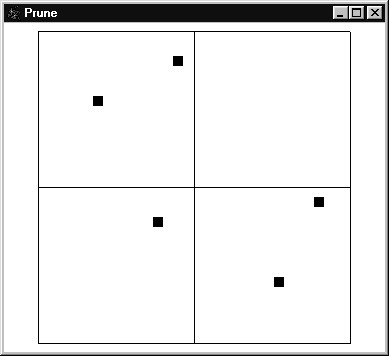
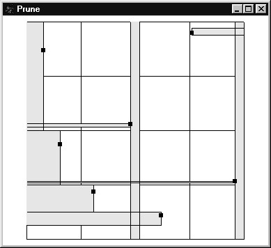
Example 1 - Obvious vertical pruning for the orbit 10010 (Figure 29 in the paper)

Click the New Periodic Orbit button, type 10010 in the Code edit box, and press OK. The periodic orbit is displayed.

The obvious vertical pruning disk is the widest disk which is symmetric about the vertical centre line and extends from top to bottom of the square. To find this disk, right-click on one of the (three) grid points on the bottom edge of the square, and select Open Out Disk from the pop-up menu. In the dialog box which appears, click on the Fill Colour button (since this figure is for export, a grayscale fill colour is appropriate) and choose a nice gray, using the Define Custom Colours button if necessary. Then click OK in the disk entry dialog box. The obvious vertical pruning disk is displayed.

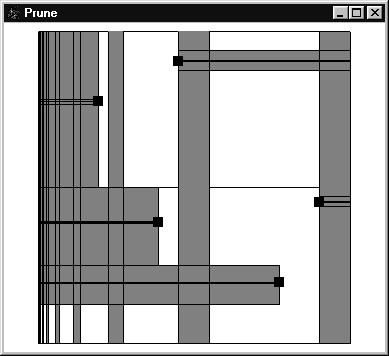
In the figure in the paper, only the iterate of the disk on the right hand edge of the square is displayed, whereas here 41 iterates in total are shown (since From and To in the New Disk dialog box were -20 and 20 respectively. Try right-clicking on the corner of one of the disks displayed, and choosing Highlight Disk from the pop-up menu. By pressing the < and > buttons, you can see how the disk behaves under the action of the horseshoe. 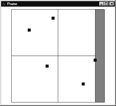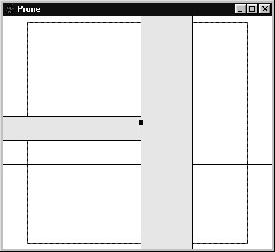Notice that iterate 0 of the disk (the one initially highlighted) is the one which is symmetric about the vertical centre line. To display just the disk against the right hand edge (which is iterate 1), right click on the corner of one of the disks, choose Edit Disk from the pop-up menu, and change both From and To to 1. (These fields can only be changed using the up-down buttons, which can be rather boring.) This produces

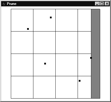
To make the figure look exactly like Figure 29 in the paper, we need one more level of grid lines (so increase the value in the Grid edit box to 2), and the points of the periodic orbit should be rather smaller. Right-click on one of the orbit points, choose Edit Orbit from the pop-up menu, and decrease Size to 3 in the dialog box which appears.

Example 2 - The Maximal pruning front relative to 1000110 (Figure 35b) in the paper)

First plot the orbit using the New Periodic Orbit button (with the plotted points of size 3), and find the obvious vertical pruning just as in Example 1. Choose a light shade of gray for the fill colour. In the version below, I've taken From and To to be 0 and 8 respectively.

Clearly this disk couldn't have been taken wider because it's run into the periodic point on its left hand edge (the point of the orbit closest to the centre of the square). We therefore choose to open out the next pruning disk to the height of this periodic point. Since it's not on the unstable manifold of 0 this isn't permitted - but the top corner of the 7th iterate of the pruning disk will do just as well. Zoom in to a small region around the periodic point in question by dragging with the left mouse button pressed.

Right click on the corner of the 7th iterate just above the periodic point, and choose Open Out Disk. Select a slightly darker shade of gray, and set From and To to -1 and 1 respectively. Click OK, and then Zoom Out from the control window.

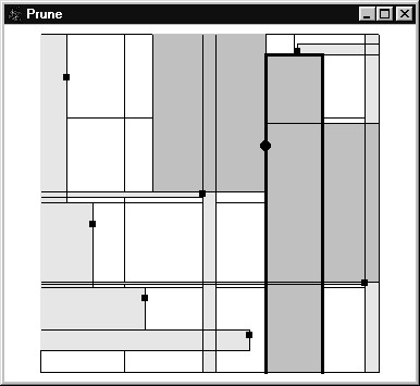
This pruning disk is maximal because it has run into the fixed point of code 1: if it were any wider then it would violate the pruning condition. You can see this by clicking New Periodic Orbit, entering the Code 1, and choosing size 5 and a solid circle style to distinguish the fixed point from the periodic orbit.

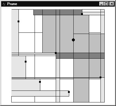
In order to avoid violating the pruning condition with respect to the -1st iterate of the pruning disk just added (highlighted in the figure above), the next pruning disk should only extend down to the top of this disk. Right-click one of the corners of this -1st iterate, choose Open Out Disk, select a still darker shade of gray, and set From and To to be 0 and 1 respectively.

To get Figure 35b) exactly, right-click on one of the corners of the second pruning disk, and change From from -1 to 0 in the Edit Disk dialog box. (It was necessary to show the -1st iterate initially, in order to know how deep to open out the final pruning disk. It should be noted, though, that the program takes account of all iterates of a pruning disk when calculating how far another disk can be opened out, not just those which are displayed. Thus, for instance, had we taken From to be 0 when this disk was originally plotted, and then tried to open out a disk to just above the fixed point, the new disk would have been contained in those already plotted.)

Click on Export EPS, choose a filename, and you're ready to include this figure in your own documents.

The homeomorphism obtained by pruning each of the three pruning disks in this example is the pseudo-Anosov in the isotopy class of the horseshoe relative to the periodic orbit in question (up to a semi-conjugacy collapsing wandering domains). A Markov partition for this pseudo-Anosov can be determined from the figure. (The same is true for example 1.)

Contents