

Magnetometers are used in smart phones and other devices - primarily to give orientation and direction. These are 3-axis magnetometers which measure three orthogonal components of the magnetic field (say North, East and Down). By summing the squares of these components, the total field H can be found and this is the quantity which will reveal details of shipwrecks below the sea,... For marine use, a measurement time of a second or two is sufficient.
Most such magnetometers are Hall Effect and have a precision of around a few hundred nT. The earth's magnetic field is around 50000nT and for effective wreck detecting at sea, a precision of better than 100 nT is needed. An accuracy of 10nT would be sufficient to provide a similar capability to a proton magnetometer.
A magnetometer on a chip with 3-axis measurement is readily available and not very expensive. The optimum technology at present seems to be non-linear inductive measurement: basically a circuit charges a coil with a magnetic core and then discharges it, measuring the time taken. If the coil core has a magnetic material with a non-linear permeability, the time taken depends on the total field and so the field can be measured. By comparing the time taken in one sense (direction) with that in the opposite sense, the difference depends on the external (earth's) magnetic field.
Such techniques are used by the RM3100 board made by PNI Corp. This sells for around $20 in the US and gives output accurate to 10 nT or so.
For an evaluation (for potential use on a satellite) of this board, see here. This describes the requirements to achieve an accuracy of a few nT. To achieve such an accuracy, it was necessary to shield the RM3100 effectively from electrical interference - and a "copper room" was found to be effective.
My proton magnetometer is very bulky and towing it behind the boat is often inconvenient. Also it cannot cope with a strongly varying field (such as over a shallow wreck - though Caesium vapour magnetometers can cope with that). Furthermore, the signal from the proton magnetometer head is a very weak analogue signal at around 1 kHz - which is very difficult to keep noise-free in a boat with a big alternator attached to the engine. So, I decided to investigate the possibility of using the RM3100 as a marine magnetometer.
This I2C access has to be by using digital signals from a computer and I set up an Arduino Uno for that. This is relatively straightforward except that the Arduino Uno is 5volt [though some Arduino models are 3.5volt] whereas the RM3100 is 3.5volt. I used a bi-directional level-shifter (Sparkfun BOB-12009) to deal with this mismatch. The level-shifter has an additional small advantage - it can drive the I2C bus with more current - so an I2C cable length of a few metres might be achievable.
Initial results were rather unpromising - until I discovered that some of the pin-heads on the wires I used to join the boards on my test-bed were magnetic.
Another cause for concern is obtaining the total magnetic field in a
moving boat from the three components measured. The RM3100 board averages over
a number C of cycles to obtain the results that can be read from the
registers. During this averaging period, the board will move and change
attitude (since the boat rolls, pitches and yaws). The average of these
components Hx, Hy and Hz will not give the true average total H. Since
sqrt(<Hx>2 +<Hy>2 +<Hz>2 ) =/= <H>
because of the fluctuations. Another bias comes from the sequential
measurement (by the chip) of the x, y and z components - so they will not be
measured simultaneously. I wrote a computer program to model this - assuming a
sinusoidal roll by +/- 20° with period 3 seconds (this is at the extreme
end of discomfort on a small boat). For example, if the averaging period
(during which all 3 components are measured in sequence) was 25ms, I found
that any bias was largest ( 0.6% ) when the field is at 45° to the x and z
axes. This bias is 270nT and can have either sign.
This is relevant since increasing cycle count C also results in additional
gain (nT per LSB - so accuracy of signal reported) but with longer averaging
times. In order to have optimum resolution C = 400 or 800 is required: these
values have gain 6.67 and 3.33 nT/LSB and take 13 and 26 ms respectively for a
measurement (average of C cycles of all three components).
I initially chose C=800 since it gives a 3nT digital accuracy and then
averaged over 32 such measurements (total time 0.8 sec). This value is then
saved to my laptop (if connected) and also output as a NMEA0183 sentence
(containing the 5 digit magnetic field strength in nT) to a data-logger.
Images of the magnetometer head (soldered to a 4-way cable) and the
driving Arduino with level-shifter.
Arduino code for RM3100 - here (sample code - no guarantee that it's bug-free)
Calibration To check out the magnetometer, I saved the 3-axis readings from every measurement to my laptop (using "screen -L") and then analysed them using a (Fortran) program. Since I only have access to the earth's field as a suitable source, I rotated the magnetometer head to many different orientations at one location and then checked whether the total magnetic field was constant.
Possible biases are (i) offsets (from permanent magnetisation on board etc) (ii) effects of induced magnetism on board (iii) scale shifts (from z-axis having different sensitivity from x and y, for example) (iv) non-orthogonal axes (z not vertical with reference to the x-y plane, for example) (v) from time averaging of measured components (discussed above).
At fixed orientation, I found a s.d. (standard deviation) of 31nT
in a location where total field was around 48000 nT. This was a promising
result, since after averaging over 1 second, the error should be reduced to
around 6nT - a very useful accuracy.
As the magnetometer head was rotated this reading changed
significantly - with a s.d. of 890 nT which is indicative of significant
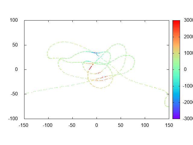
biases. As well as statistical tests, I also plotted (using Gnuplot) the total
measured magnetic field over the sphere of possible directions of the field
relative to the sensor. After invoking offsets (typically 50-200 nT) and a
scale change (of 2% in the z-direction), this spread was reduced to a s.d. of
650 nT.
The largest source of induced magnetism on the board is the coils themselves. They are solenoidal and have a high-permeability rod-shaped core. That shape will preferentially be magnetised along the long axis. So, for example, the x-component of the earth's field will induce a dipole in the x-coil. This induced dipole will have a magnetic field which has a component along the direction of the y-coil (from the geometry of the coils on the board). This implies that the y-measurement will have a small extra component from the x-component of the earth's field. Basically, there is a mutual inductance between the coils. I parametrized the 3 such mutual inductances and found a significant reduction in s.d.. Typical relative contributions are at about 0.7%.
I also explored possible effects of
non-orthogonality (eg z coil having some small x and y component). This is a
plausible scenario since the magnetometer was originally designed as a digital
compass so x-y features were original. The z-coil was added later - and stands
up like a mini-tower-block on the chip. It the tower leans at 1° to the
vertical (w.r.t x and y) then an admixture of about 2% of the x-component will
be added to the z-component (if it leans in the x-direction). Separating this
effect from the mutual inductance effect is not easily achieved - since it
increases the cross-talk parameters from 3 to 6.
So in total 12 degrees of freedom which makes it
harder to explore all possibilities.
To find the optimum offsets and other parameters, I
minimized the sum over data of (data-true)^2 where the offsets, etc are
applied to the data and "true" is the average value of the total field:
so basically the variance of the data after correction (square of s.d.).
Another possible source of error is from reading results while the head is
rotating. I checked this by selecting those results which have successive
directions (of the magnetic field relative to the sensor) which are close (say
less than 0.25° apart). From the measured magnetic field vectors
h=(h
A way to partially correct for this effect of rotational motion is to save separately the x,y and z components measured and then interpolate each of them in time - so allowing to get the three components at a common time. This helps significantly: linear interpolation reduced the s.d. from 650nT to 360nT.
To investigate again the fixed biases, I measured the field in the same location with the sensor held fixed in a series of different attitudes. The raw data for the intensity has a spread with s.d. of 655nT, but after selecting offsets, scaling and parmetrizing the mutual induction (9 parameters in total - so quite an art to get the best fit), this reduces to 74nT. This is a substantial improvement but it is still larger than the result from a single fixed position (31nT).
Using linear interpolation in time, as discussed above, I got raw s.d. of 650nT and with optimum corrections included this reduced to only 86nT. Restricting to orientations of the magnetometer board which were only about 20° from vertical: then raw was 298nT and, with the same corrections, the s.d. was 67nT.
By only retaining data with a less than 1° (240/14000) change in direction of the field between successive measurements (25ms), the s.d can be reduced a bit further (to 72 and 62 resp) but with a significant fraction of the data excluded.
Include MPU6050 board to give 3-axis accelerometer and gyro input. Write custom code to combine inputs to give gravity vector in sensor coordinates. This allows Hz (vertical component of H, namely H.G where G is gravity (unit) direction) to be determined (as well as total H) which may help in interpretation of anomalies. It also allows Ht (transverse component to vertical) to be determined.
Combine MPU board and RM3100 board on opposite ends of a circuit board and fit in plastic housing. Output LCD and NMEA0183.
Combined board:
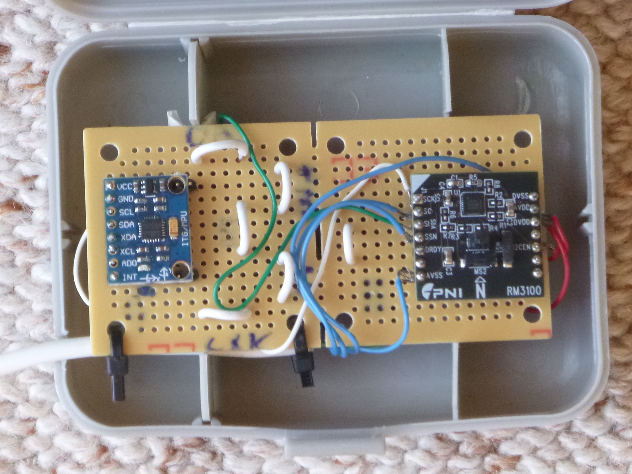
Issues: result depends on orientation (range 500 nT). This seems to be from combining boards. Also some meta-stability: result stable but changes after jiggling leads. Also some sign that power to MPU board affects magnetic results.
Test at sea - signal over shallow wreck. Issues with directional offsets and stability. Also with Hz negative (box inverted?). Stbd berth seems slightly preferable to port berth.
Results from a first test over a shallow wreck in the Rock Channel: image, showing nice signal.
Options: test in garden; solder Uno and level-shifter connections; new RM3100; [in progress]